Contents
Morphometrics and physical markers
Morphometrics (morpho– shape; metrics– measurements) is the use of physical measurements to determine the relatedness of organisms. With extinct organisms that have died out long ago, DNA extraction proves to be difficult. Likewise, prior to DNA technologies to analyze species, Linnean taxonomy was ascribed to organisms based on similarities in features.
Describing Species and Variation of Morphologies
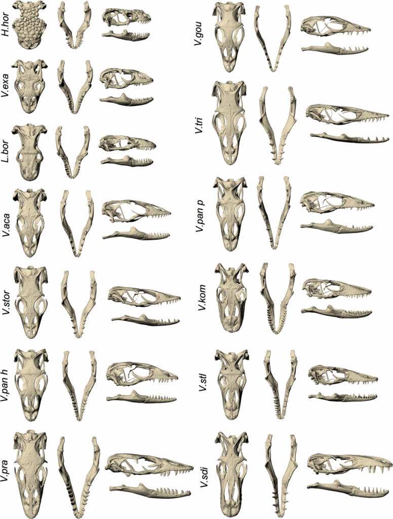
Below are images of skull landmarks of the lizard family Varanidae. This family includes monitor lizards and Komodo Dragons.As can be seen below, the general morphology of the skulls are similar enough that they all retain the same landmarks. The figure below also illustrates the diversity in these lizards that illustrate a large variety between species.

Skulls of the species involved in this analysis. McCurry et al. (2015) (CC-BY)
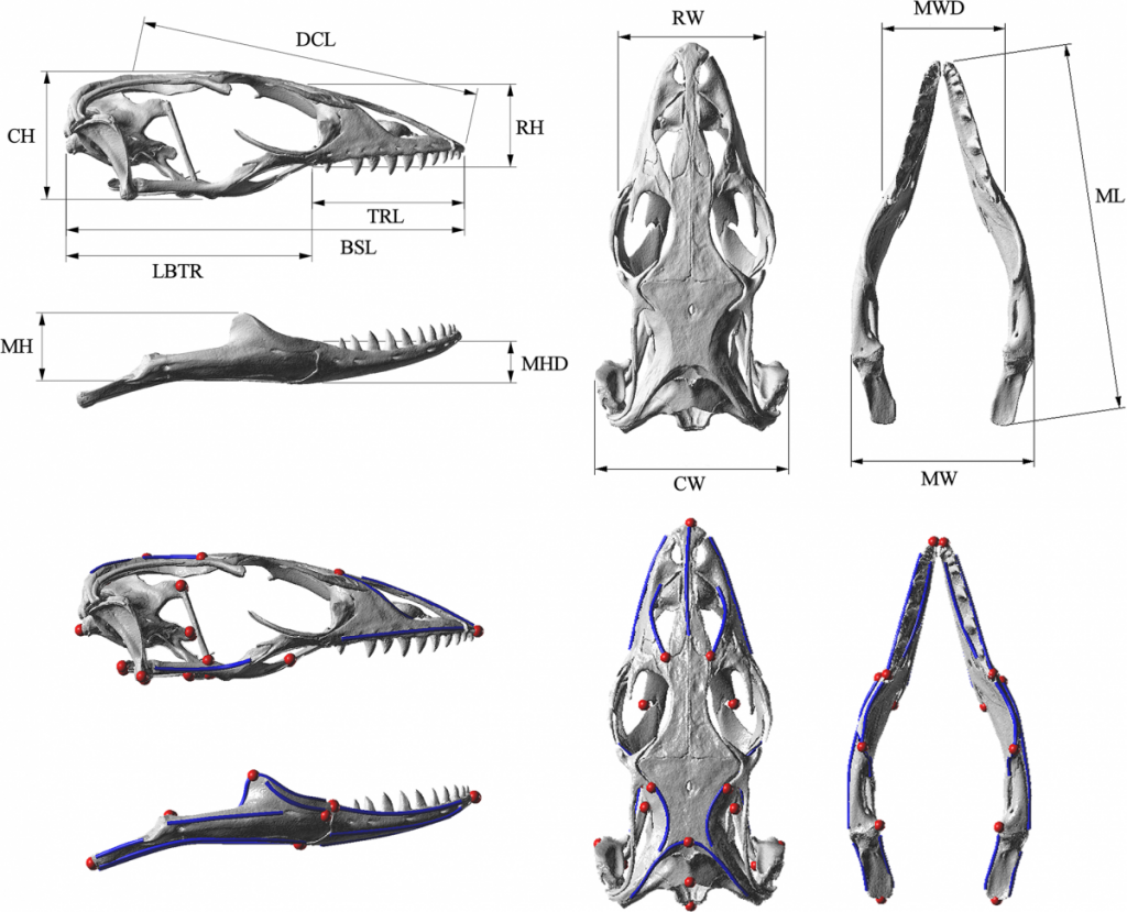
Landmarks Standardize measurements
Having a set of shared landmarks provides the opportunity to make systematic measurements of morphometric features.

Landmarks and measurement metrics for the morphometric analysis of skulls. McCurry et al. (2015) (CC-BY)
Euclidean distance is a measurement derived from Pythagorean geometry that describes the shortest distance (d) between 2 points (A & B) as a straight line using triangulation. In a cartesian space, the points can be defined:
and
Standard pythagorean theorem can be expressed as:
To find the distance between the 2 points, we utilize algebra to calculate for .
In this case, we expand to comparing the coordinates of the two points:
and
We can then expand this idea to include the differences of data points that describe the comparisons of multiple measurements.
Calculating distance with R

- Download the dataset (McCurry et al. 2015) associated with this activity (a Comma Separated Value .csv file). This can be used in a spreadsheet or in a text editor. This data can be imported into R to determine the euclidean distances of landmarks.
- The following code in R will download the data set into a variable called “varanoid”, measure euclidean distance and save a plot into a PDF file in a directory called “/tmp”.
## install curl for fetching from internet if it isn't
install.packages('curl')
## Load the curl library
library(curl)
## read the data of measurements and assign it to a variable 'varanoid'
varanoid = read.csv(curl('https://raw.githubusercontent.com/jeremyseto/bio-oer/master/data/varanoid.csv'))
## set the row names to the Species column
row.names(varanoid) = varanoid$Species
## remove the first column of the table to have purely numeric data
varanoid_truncated = (varanoid[,2:14])
## calculate distance using euclidean as the method
dist_measure = dist(varanoid_truncated, method='euclidean')
## display dist_measure to look at the comparisons
dist_measure
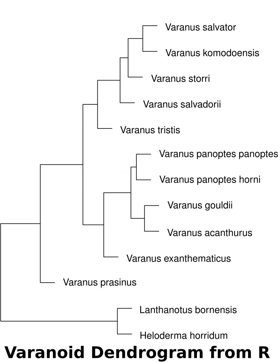
varanoid_cluster = hclust(dist_measure)
## open PDF as a graphics device  to save a file in the '/tmp' directory
pdf(file='/tmp/varanoid_tree.pdf')
plot(varanoid_cluster)
dev.off()
## close the device to save the plot as pdf
DNA Analysis
Before starting this activity, review bioinformatics and sequence analysis.
- Search NCBI for mitochondrial sequences from the species involved in McCurry 2015. The data has been submitted by Ast (2001).
- Find the sequences and identify/extract elements that are common to all
- Assemble the shared sequences in a text editor as a single FASTA file where each species is separated by a header (“>Species A”)
- Notepad on Windows (but it’s better to download notepad++)
- Textedit on Mac (but probably better to download TextWrangler)
- Gedit on Linux
- Save the file as “something.fasta”
- Perform a multiple sequence analysis using UGENE
- Generate a phylogenetic tree using UGENE. For this exercise, use Maximum Likelihood (PhyML) as the algorithm. File the tutorial below.
- Compare the DNA with the morphometric analyses. What problems could we imagine arise if we rely solely on morphometry.
References
- McCurry MR, Mahony M, Clausen PD, Quayle MR, Walmsley CW, Jessop TS, Wroe S, Richards H, McHenry CR. (2015) The Relationship between Cranial Structure, Biomechanical Performance and Ecological Diversity in Varanoid Lizards. PLoS ONE 10(6): e0130625. doi: 10.1371/journal.pone.0130625
- Ast, Jennifer C. (2001) Mitochondrial DNA Evidence and Evolution in Varanoidea (Squamata). Cladistics 17(3): 211–26. http://www.sciencedirect.com/science/article/pii/S0748300701901690
- Fisher, R.A. (1936) The use of multiple measurements in taxonomic problems. Annals of Eugenics, 7: 179–188. doi:10.1111/j.1469-1809.1936.tb02137.x


